41 how to show labels in excel chart
How to add data labels from different column in an Excel chart? Right click the data series in the chart, and select Add Data Labels > Add Data Labels from the context menu to add data labels. 2. Click any data label to select all data labels, and then click the specified data label to select it only in the chart. 3. How to Add Two Data Labels in Excel Chart (with Easy Steps) Step 1: Create a Chart to Represent Data Step 2: Add 1st Data Label in Excel Chart Step 3: Apply 2nd Data Label in Excel Chart Step 4: Format Data Labels to Show Two Data Labels Things to Remember Conclusion Related Articles Download Practice Workbook Download this dataset and practice while going through this article. Add Two Data Labels.xlsx
Waterfall Chart Template - Download Free Excel Template Download the Free Template. Enter your name and email in the form below and download the free template now! A waterfall chart is a great way to visually show the effect of positive and negative cash flows on a cumulative basis. In Excel 2016, there is a built-in waterfall chart option so it is a very simple and quick process.

How to show labels in excel chart
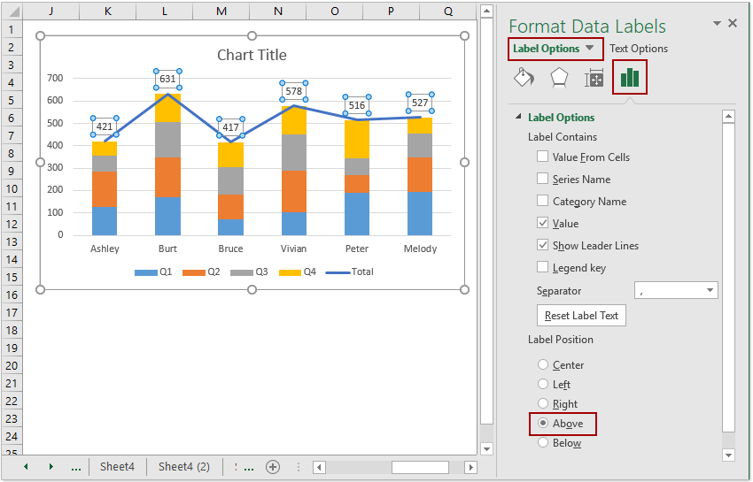
HOW TO CREATE A BAR CHART WITH LABELS ABOVE BAR IN EXCEL - simplexCT In the Format Data Labels pane, under Label Options selected, set the Label Position to Inside End. 16. Next, while the labels are still selected, click on Text Options, and then click on the Textbox icon. 17. Uncheck the Wrap text in shape option and set all the Margins to zero. The chart should look like this: 18. Edit titles or data labels in a chart - support.microsoft.com On a chart, click the label that you want to link to a corresponding worksheet cell. On the worksheet, click in the formula bar, and then type an equal sign (=). Select the worksheet cell that contains the data or text that you want to display in your chart. You can also type the reference to the worksheet cell in the formula bar. how to add data labels into Excel graphs — storytelling with data Option 2: Embedding labels directly Let's look now at an alternative approach: embedding the labels directly. You can download the corresponding Excel file to follow along with these steps: Right-click on a point and choose Add Data Label.
How to show labels in excel chart. How To Add Data Labels In Excel - life-insurance-info.us How To Add Data Labels In Excel. Click on the arrow next to data labels to change the position of where the labels are in relation to the bar chart. Change position of data labels. How to Add Data Labels in Excel Excelchat Excelchat from After picking the series, click the data point you want to label. Click the chart to show the chart elements button. Required steps to print ... How to add data labels in excel to graph or chart (Step-by-Step) Add data labels to a chart. 1. Select a data series or a graph. After picking the series, click the data point you want to label. 2. Click Add Chart Element Chart Elements button > Data Labels in the upper right corner, close to the chart. 3. Click the arrow and select an option to modify the location. 4. How To Add Data Labels In Excel - pravove-pole.info Then, click the insert tab along the top ribbon and click the insert scatter (x,y) option in the charts group. Click on the arrow next to data labels to change the position of where the labels are in relation to the bar chart. To format data labels in excel, choose the set of data labels to format. Source: How to Use Cell Values for Excel Chart Labels - How-To Geek Select the chart, choose the "Chart Elements" option, click the "Data Labels" arrow, and then "More Options." Uncheck the "Value" box and check the "Value From Cells" box. Select cells C2:C6 to use for the data label range and then click the "OK" button. The values from these cells are now used for the chart data labels.
Display Data Labels Above Data Markers in Excel Chart How to Display Data Labels Above Data Markers Method 1: Use the Chart Elements Button Method 2: Use the Add Chart Element Drop-Down List Method 3: Use the Shortcut Menu Method 4: Apply a Quick Layout Conclusion How to Display Data Labels Above Data Markers It can be difficult to understand an Excel chart that does not have data labels. How to create a chart with both percentage and value in Excel? Click OK button, then, go on right click the bar in the char, and choose Add Data Labels > Add Data Labels, see screenshot: 12. And the values have been added into the chart as following screenshot shown: 13. Then, please go on right click the bar, and select Format Data Labels option, see screenshot: 14. How to change Axis labels in Excel Chart - A Complete Guide Step-by-Step guide: How to Change Axis labels in Excel. Change the Horizontal X-Axis Labels. Method-1: Changing the worksheet Data. Method-2: Without changing the worksheet Data. Method-3: Using another Data Source. Change the format Text or Number of the Axis Labels. Show or hide Axis Labels. Add or remove data labels in a chart - support.microsoft.com Click Label Options and under Label Contains, pick the options you want. Use cell values as data labels You can use cell values as data labels for your chart. Right-click the data series or data label to display more data for, and then click Format Data Labels. Click Label Options and under Label Contains, select the Values From Cells checkbox.
How to Display Percentage in an Excel Graph (3 Methods) Then go to the More Options via the right arrow beside the Data Labels. Select Chart on the Format Data Labels dialog box. Uncheck the Value option. Check the Value From Cells option. Then you have to select cell ranges to extract percentage values. For this purpose, create a column called Percentage using the following formula: =E5/C5 How to Add Axis Labels in Excel Charts - Step-by-Step (2022) - Spreadsheeto How to add axis titles 1. Left-click the Excel chart. 2. Click the plus button in the upper right corner of the chart. 3. Click Axis Titles to put a checkmark in the axis title checkbox. This will display axis titles. 4. Click the added axis title text box to write your axis label. How to Insert Axis Labels In An Excel Chart | Excelchat In Excel 2016 and 2013, we have an easier way to add axis labels to our chart. We will click on the Chart to see the plus sign symbol at the corner of the chart Figure 9 - Add label to the axis We will click on the plus sign to view its hidden menu Here, we will check the box next to Axis title Figure 10 - How to label axis on Excel Change axis labels in a chart - Microsoft Support On the Character Spacing tab, choose the spacing options you want. To change the format of numbers on the value axis: Right-click the value axis labels you want to format. Click Format Axis. In the Format Axis pane, click Number. Tip: If you don't see the Number section in the pane, make sure you've selected a value axis (it's usually the ...
Is there a way to show different data labels in a bar chart ...
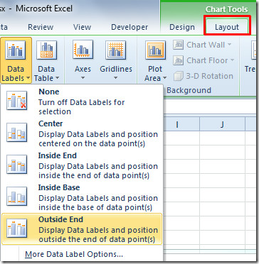
How to add or move data labels in Excel chart? - ExtendOffice In Excel 2013 or 2016 1. Click the chart to show the Chart Elements button . 2. Then click the Chart Elements, and check Data Labels, then you can click the arrow to choose an option about the data labels in the sub menu. See screenshot: In Excel 2010 or 2007 1. click on the chart to show the Layout tab in the Chart Tools group. See screenshot: 2.

Directly Labeling Your Line Graphs | Depict Data Studio
How to hide zero data labels in chart in Excel? - ExtendOffice Right click at one of the data labels, and select Format Data Labelsfrom the context menu. See screenshot: 2. In the Format Data Labelsdialog, Click Numberin left pane, then selectCustom from the Categorylist box, and type #""into the Format Codetext box, and click Addbutton to add it to Typelist box. See screenshot: 3.

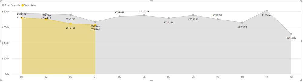
How to add live total labels to graphs and charts in Excel ...
How to use data labels in a chart - YouTube Excel charts have a flexible system to display values called "data labels". Data labels are a classic example a "simple" Excel feature with a huge range of o...

How to Get Colors in Excel Chart Data Lables - Formatting Trick
Excel: How to Create a Bubble Chart with Labels - Statology To add labels to the bubble chart, click anywhere on the chart and then click the green plus "+" sign in the top right corner. Then click the arrow next to Data Labels and then click More Options in the dropdown menu: In the panel that appears on the right side of the screen, check the box next to Value From Cells within the Label Options group:

How to Add Two Data Labels in Excel Chart (with Easy Steps ...
Change the format of data labels in a chart - Microsoft Support To get there, after adding your data labels, select the data label to format, and then click Chart Elements > Data Labels > More Options. To go to the appropriate area, click one of the four icons ( Fill & Line, Effects, Size & Properties ( Layout & Properties in Outlook or Word), or Label Options) shown here.

Display Customized Data Labels on Charts & Graphs
how to add data labels into Excel graphs — storytelling with data Option 2: Embedding labels directly Let's look now at an alternative approach: embedding the labels directly. You can download the corresponding Excel file to follow along with these steps: Right-click on a point and choose Add Data Label.
Excel 2010: Show Data Labels In Chart
Edit titles or data labels in a chart - support.microsoft.com On a chart, click the label that you want to link to a corresponding worksheet cell. On the worksheet, click in the formula bar, and then type an equal sign (=). Select the worksheet cell that contains the data or text that you want to display in your chart. You can also type the reference to the worksheet cell in the formula bar.
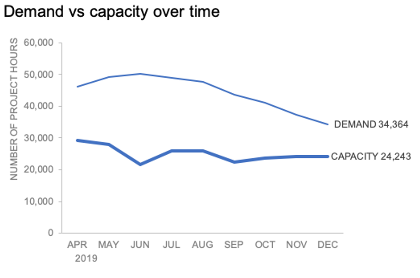
Label line chart series
HOW TO CREATE A BAR CHART WITH LABELS ABOVE BAR IN EXCEL - simplexCT In the Format Data Labels pane, under Label Options selected, set the Label Position to Inside End. 16. Next, while the labels are still selected, click on Text Options, and then click on the Textbox icon. 17. Uncheck the Wrap text in shape option and set all the Margins to zero. The chart should look like this: 18.

Excel charts: add title, customize chart axis, legend and ...
Move and Align Chart Titles, Labels, Legends with the Arrow ...
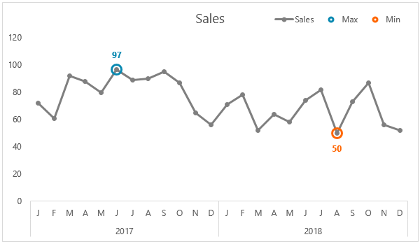
Label Excel Chart Min and Max • My Online Training Hub

How-to Add Label Leader Lines to an Excel Pie Chart - Excel ...
how to add data labels into Excel graphs — storytelling with data

How to add or move data labels in Excel chart?
How to show the percentage on stacked colum/bar chart in ...

Custom data labels in a chart

charts - Excel, giving data labels to only the top/bottom X ...

How to Add Axis Labels to a Chart in Excel | CustomGuide

How to show data labels in PowerPoint and place them ...

Excel charts: add title, customize chart axis, legend and ...

Total of chart series – Excel kitchenette

Excel sunburst chart: Some labels missing - Stack Overflow
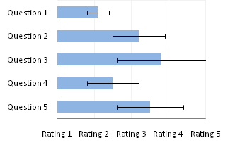
Text Labels on a Horizontal Bar Chart in Excel - Peltier Tech

Improve your X Y Scatter Chart with custom data labels

Add or remove data labels in a chart - Microsoft Support

How to Use Cell Values for Excel Chart Labels

Dynamic Number Format for Millions and Thousands - PK: An ...

Adding rich data labels to charts in Excel 2013 | Microsoft ...

microsoft excel - Adding data label only to the last value ...

Chart axes, legend, data labels, trendline in Excel - Tech Funda

microsoft excel - Adding data label only to the last value ...
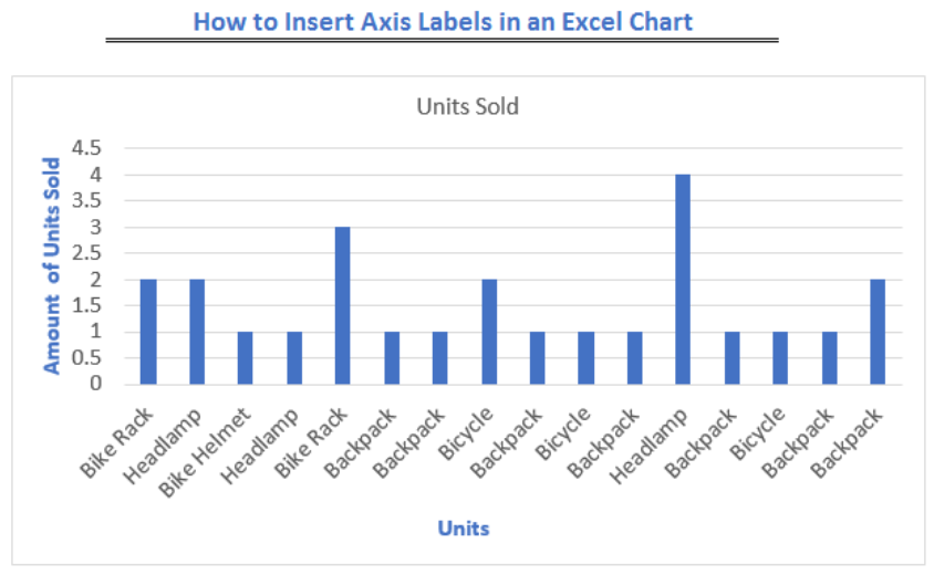
How to Insert Axis Labels In An Excel Chart | Excelchat

Add Labels ON Your Bars
Solved: Area chart data labels not in correct positions ...

How-to Use Data Labels from a Range in an Excel Chart - Excel ...

How To Show Or Hide Data Labels On MS Excel? | My Windows Hub

Enable or Disable Excel Data Labels at the click of a button ...
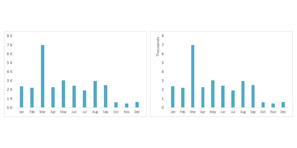
Show numbers in thousands in Excel as K in table or chart
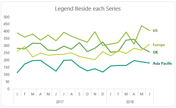
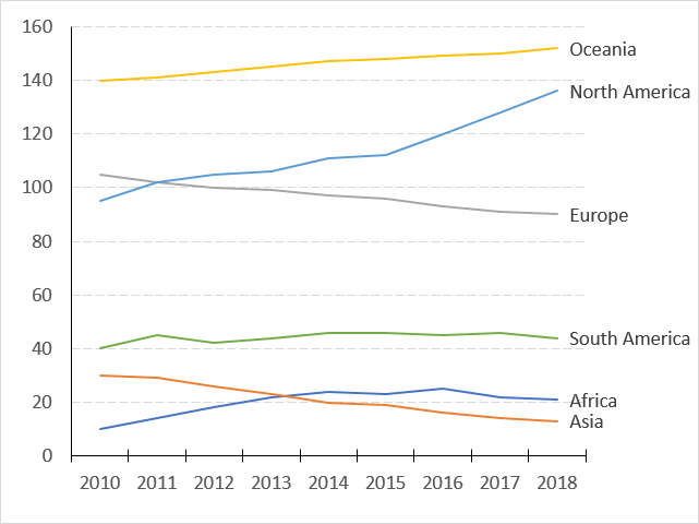
Dynamically Label Excel Chart Series Lines • My Online ...
How to add total labels to stacked column chart in Excel?

Add or remove data labels in a chart - Microsoft Support
Post a Comment for "41 how to show labels in excel chart"