41 excel scatter diagram with labels

Add labels to scatter graph - Excel 2007 | MrExcel Message Board Nov 10, 2008. #1. OK, so I have three columns, one is text and is a 'label' the other two are both figures. I want to do a scatter plot of the two data columns against each other - this is simple. However, I now want to add a data label to each point which reflects that of the first column - i.e. I don't simply want the numerical value or ... Improve your X Y Scatter Chart with custom data labels - Get Digital Help Select the x y scatter chart. Press Alt+F8 to view a list of macros available. Select "AddDataLabels". Press with left mouse button on "Run" button. Select the custom data labels you want to assign to your chart. Make sure you select as many cells as there are data points in your chart. Press with left mouse button on OK button. Back to top

How to use a macro to add labels to data points in an xy scatter chart ... In Microsoft Office Excel 2007, follow these steps: Click the Insert tab, click Scatter in the Charts group, and then select a type. On the Design tab, click Move Chart in the Location group, click New sheet , and then click OK. Press ALT+F11 to start the Visual Basic Editor. On the Insert menu, click Module.

Excel scatter diagram with labels

The Problem With Labelling the Data Points in an Excel Scatter Chart Labelling the data points in an Excel chart is a useful way to see precise data about the values of the underlying data alongside the graph itself. In a column chart, for instance, you might show the value of the data point at the top of a column. A useful addition to a column chart is a set of data labels showing the value of each column. Excel scatter chart using text name - Access-Excel.Tips Scatter chart is used to display the actual data point, while bar chart is to display Grade labels. - Create scatter chart for Range B20:C31 (Series 1) - Add bar chart (column chart) for Range F20:G26 (Series 2) Due to 0 y axis for Series 2, no value is displayed, only the x-axis label can be seen. The outcome should look like below. Labeling points in excel scatter diagram - YouTube Showing how to put labels on points of an excel scatter diagram. The video can help familiarize with plotting a scatter diagram, putting trendlines, formatting the chart, x and y axis, use of...

Excel scatter diagram with labels. How To Create Scatter Chart in Excel? - EDUCBA To apply the scatter chart by using the above figure, follow the below-mentioned steps as follows. Step 1 - First, select the X and Y columns as shown below. Step 2 - Go to the Insert menu and select the Scatter Chart. Step 3 - Click on the down arrow so that we will get the list of scatter chart list which is shown below. Excel 2019/365: Scatter Plot with Labels - YouTube How to add labels to the points on a scatter plot. Use text as horizontal labels in Excel scatter plot Edit each data label individually, type a = character and click the cell that has the corresponding text. This process can be automated with the free XY Chart Labeler add-in. Excel 2013 and newer has the option to include "Value from cells" in the data label dialog. Format the data labels to your preferences and hide the original x axis labels. How to Add Labels to Scatterplot Points in Excel - Statology Step 1: Create the Data First, let's create the following dataset that shows (X, Y) coordinates for eight different groups: Step 2: Create the Scatterplot Next, highlight the cells in the range B2:C9. Then, click the Insert tab along the top ribbon and click the Insert Scatter (X,Y) option in the Charts group. The following scatterplot will appear:

How to quickly create bubble chart in Excel? - ExtendOffice 5. if you want to add label to each bubble, right click at one bubble, and click Add Data Labels > Add Data Labels or Add Data Callouts as you need. Then edit the labels as you need. If you want to create a 3-D bubble chart, after creating the basic bubble chart, click Insert > Scatter (X, Y) or Bubble Chart > 3-D Bubble. Create a Pareto Chart in Excel (In Easy Steps) - Excel Easy If you don't have Excel 2016 or later, simply create a Pareto chart by combining a column chart and a line graph. This method works with all versions of Excel. 1. First, select a number in column B. 2. Next, sort your data in descending order. On the Data tab, in the Sort & Filter group, click ZA. 3. Calculate the cumulative count. Excel 2016 - Personalised labels for XY scatter plot 1. Select the first XY pair and create the scatter chart (using the icon). 2. Then use the "Select Data" dialog (right click on the chart) to change the series as follows: 2a: change the name of the series to the cell reference for the label for that XY pair. 2b: change the X-value to the X-cell reference for the XY pair. Hover labels on scatterplot points - Excel Help Forum Hi Everyone, I am hoping someone can point me in the right direction on a challenge I am trying to solve. I have data on an xy scatterplot and would like to be able to move by mouse over the points and have a label show up for each point showing the X,Y value of the point and also text from a comment cell. I know excel has these hover labels but i cant seem to find a way to edit them.

Creating Scatter Plot with Marker Labels - Microsoft Community Hi, Create your scatter chart using the 2 columns height and weight. Right click any data point and click 'Add data labels and Excel will pick one of the columns you used to create the chart. Right click one of these data labels and click 'Format data labels' and in the context menu that pops up select 'Value from cells' and select the column ... Scatter Plot in Excel (In Easy Steps) - Excel Easy To create a scatter plot with straight lines, execute the following steps. 1. Select the range A1:D22. 2. On the Insert tab, in the Charts group, click the Scatter symbol. 3. Click Scatter with Straight Lines. Note: also see the subtype Scatter with Smooth Lines. Result: Note: we added a horizontal and vertical axis title. Find, label and highlight a certain data point in Excel ... Oct 10, 2018 · Select the Data Labels box and choose where to position the label. By default, Excel shows one numeric value for the label, y value in our case. To display both x and y values, right-click the label, click Format Data Labels…, select the X Value and Y value boxes, and set the Separator of your choosing: Label the data point by name How to Make a Scatter Plot in Excel with Two Sets of Data? - PPCexpo To get started with the Scatter Plot in Excel, follow the steps below: Open your Excel desktop application. Open the worksheet and click the Insert button to access the My Apps option. Click the My Apps button and click the See All button to view ChartExpo, among other add-ins.

Placing labels on data points in a stacked bar chart in Excel - Super User

How to plot a ternary diagram in Excel - Chemostratigraphy.com Feb 13, 2022 · Insert a Scatter Chart (XY diagram), e.g., ‘Scatter with Straight Lines’ (Figure 9) using the XY coordinates for the triangle from columns AA and AB. To make it into an equilateral triangle resize the chart area accordingly; for example 10 columns wide and 30 rows high, as in Figure 10.

How to Create a Scatter Plot in Excel

How to Create Venn Diagram in Excel – Free Template Download First, let’s add data labels. Right-click on the data marker representing Series “Pepsi” and choose “Add Data Labels.” Step #15: Customize data labels. Replace the default values with the custom labels you previously designed. Right-click on any data label and choose “Format Data Labels.” Once the task pane pops up, do the following:

Scatter Diagrams | Scatter Graph Charting Software | Scatter Graph | Scatter Graph

X-Y Scatter Plot With Labels Excel for Mac Excel for Mac doesn't seem to support the most basic scatter plot function - creating an X-Y plot with data labels like in the simplistic example attached. Can someone please point me towards a macro which can do this? Thank you very much in advance. Labels: Charting Excel on Mac Tags: Excel for Mac Screenshot 2020-04-04 22.58.01.png 105 KB

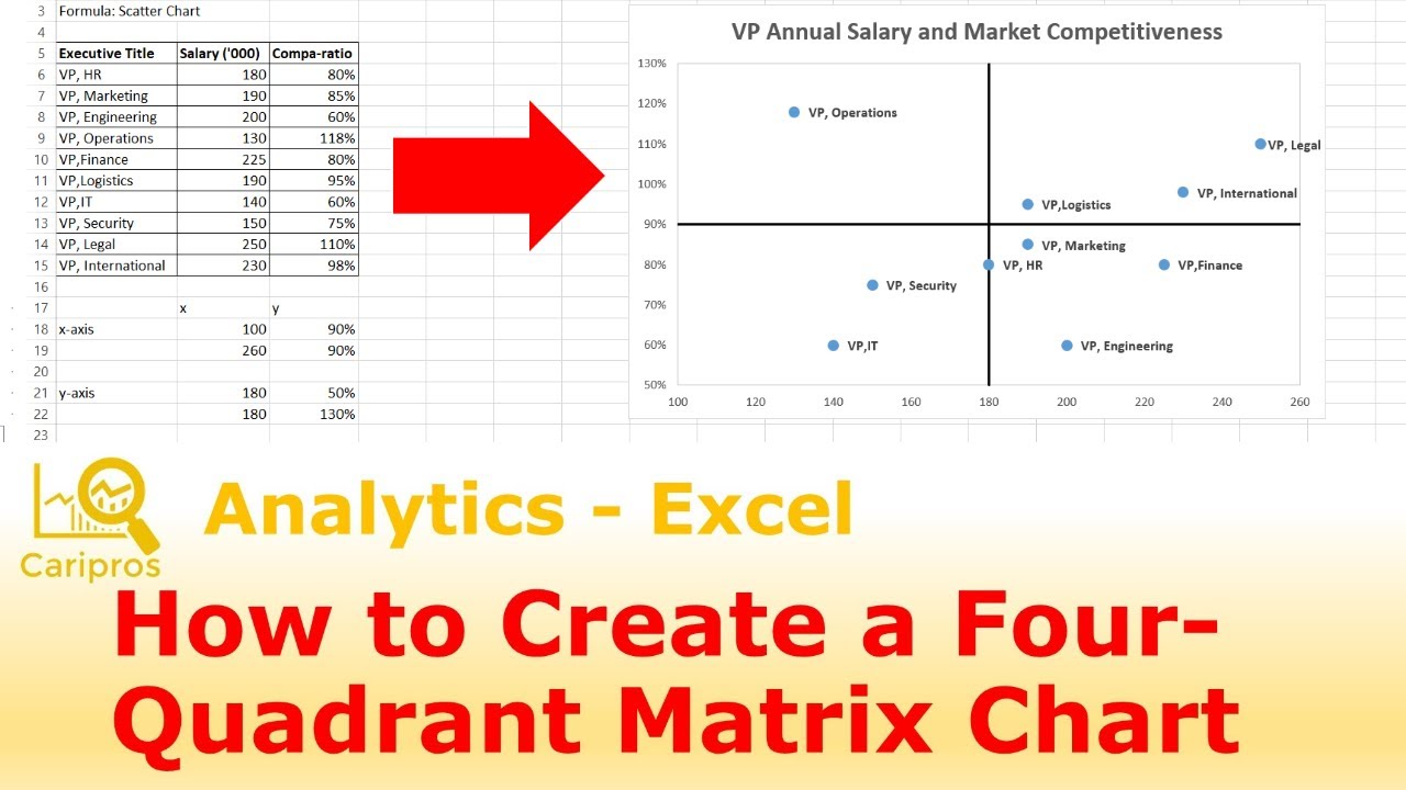
How to create a 4-Quadrant Matrix Chart in Excel - YouTube

Excel Scatter Chart with Labels - Super User Create scatter plots by selecting two column at a time and insert scatter (plot). Clicking on the button, which will add labels. Easy. Thanks to the folks that made it and recommended it. Share Improve this answer edited Sep 21, 2014 at 19:06 Mokubai ♦ 84.7k 25 195 217 answered Sep 21, 2014 at 13:54 timtak 167 1 5 Add a comment Your Answer

vba excel scatter chart - YouTube

How to Make a Scatter Plot in Excel | GoSkills How to make a scatter plot in Excel Let's walk through the steps to make a scatter plot. Step 1: Organize your data Ensure that your data is in the correct format. Since scatter graphs are meant to show how two numeric values are related to each other, they should both be displayed in two separate columns.

Best Excel Tutorial - Stiff Diagram

Scatter Diagram Help | BPI Consulting If you do, the program will add these as the labels for the X axis and Y axis. 2. Select "Scatter" from the "Cause and Effect" panel on the SPC for Excel ribbon. 3. The input screen for the scatter diagram is displayed. The program sets the initial X and Y ranges as the range that is selected on the worksheet.

Share :