42 excel pivot table labels
Pivot table row labels in separate columns • AuditExcel.co.za Our preference is rather that the pivot tables are shown in tabular form (all columns separated and next to each other). You can do this by changing the report format. So when you click in the Pivot Table and click on the DESIGN tab one of the options is the Report Layout. Click on this and change it to Tabular form. Use column labels from an Excel table as the rows in a Pivot Table Highlight your current table, including the headers Then from the Data section of the ribbon, select From Table Highlight all the columns containing data, but not the Year column, and then select Unpivot Columns Close the dialog and keep the changes. Excel should place the unpivoted data into a new worksheet, looking something like this:
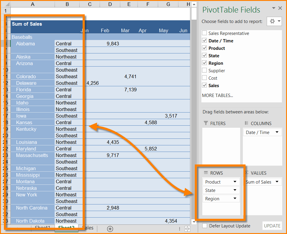
Pivot Table Row Labels - Microsoft Community If you go to PivotTable Tools > Analyze > Layout > Report Layout > Show in Tabular Form, your column headers will be used for the row labels. Every once in a while there's a sudden gust of gravity... Report abuse 1 person found this reply helpful · Was this reply helpful? Yes No A. User Replied on December 19, 2017

Excel pivot table labels
Excel Pivot Table Filter and Label Formatting - Microsoft Tech Community Excel Pivot Table Filter and Label Formatting Excel 2016 Images of 2 separate workbooks, each with a data table, pivot table and pivot chart, the one on the right created by copy & paste of the one on the left. The one on the right changed: X axis labels on the pivot chart don't have the multi-level option. How to reset a custom pivot table row label Now go back to your Pivot and refresh it to find the Problem column and the duplicate column you just made. 5. Enter both fields into the pivot table and you will see the duplicate column has the original values while the Problem column maintains the problem labels. Monday, April 27, 2015 8:39 AM 0 Sign in to vote How to Use Label Filters for Text in the Pivot Table? - MS Excel ... When you select the field name, the selected field name will be inserted into the pivot table. Pro Tip. Row Labels are used to apply a filter to rows that have to be shown in the pivot table. By default, it will show you the sum or count values in the pivot table.
Excel pivot table labels. Excel 2016 Pivot table Row and Column Labels - Microsoft Community In Excel 2016 I've found when I create a pivot table it unhelpfully shows 'Row Labels' and 'Column Labels' instead of my field names, although in the top left cell it says 'Count of' and then inserts the correct field name. Years ago when I last used Excel it automatically put the field names in all three heading cells. How to Use Excel Pivot Table Label Filters Right-click a cell in the pivot table, and click PivotTable Options. In the PivotTable Options dialog box, click the Totals & Filters tab In the Filters section, add a check mark to 'Allow multiple filters per field.' Click the OK button, to apply the setting and close the dialog box. Quick Way to Hide or Show Pivot Items Remove row labels from pivot table • AuditExcel.co.za Click on the Pivot table. Click on the Design tab. Click on the report layout button. Choose either the Outline Format or the Tabular format. If you like the Compact Form but want to remove 'row labels' from the Pivot Table you can also achieve it by. Clicking on the Pivot Table. Clicking on the Analyse tab. Data Labels in Excel Pivot Chart (Detailed Analysis) 7 Suitable Examples with Data Labels in Excel Pivot Chart Considering All Factors 1. Adding Data Labels in Pivot Chart 2. Set Cell Values as Data Labels 3. Showing Percentages as Data Labels 4. Changing Appearance of Pivot Chart Labels 5. Changing Background of Data Labels 6. Dynamic Pivot Chart Data Labels with Slicers 7.
How to Move Excel Pivot Table Labels Quick Tricks To move a pivot table label to a different position in the list, you can use commands in the right-click menu: Right-click on the label that you want to move Click the Move command Click one of the Move subcommands, such as Move [item name] Up The existing labels shift down, and the moved label takes its new position. Type Over Another Label Design the layout and format of a PivotTable In the PivotTable Options dialog box, click the Layout & Format tab, and then under Layout, select or clear the Merge and center cells with labels check box. Note: You cannot use the Merge Cells check box under the Alignment tab in a PivotTable. Change the display of blank cells, blank lines, and errors Pivot table row labels side by side - Excel Tutorials You can copy the following table and paste it into your worksheet as Match Destination Formatting. Now, let's create a pivot table ( Insert >> Tables >> Pivot Table) and check all the values in Pivot Table Fields. Fields should look like this. Right-click inside a pivot table and choose PivotTable Options…. Check data as shown on the image below. Repeat item labels in a PivotTable - support.microsoft.com Repeating item and field labels in a PivotTable visually groups rows or columns together to make the data easier to scan. For example, use repeating labels when subtotals are turned off or there are multiple fields for items. In the example shown below, the regions are repeated for each row and the product is repeated for each column.
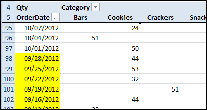
Automatic Row And Column Pivot Table Labels - How To Excel At Excel Select the data set you want to use for your table The first thing to do is put your cursor somewhere in your data list Select the Insert Tab Hit Pivot Table icon Next select Pivot Table option Select a table or range option Select to put your Table on a New Worksheet or on the current one, for this tutorial select the first option Click Ok Turn Repeating Item Labels On and Off - Excel Pivot Tables To change the setting: Right-click one of the items in the field - in this example I'll right-click on "Cookies". In the pop-up menu, click Field Settings. In the Field Settings window, click the Layout & Print tab. Add a check mark to Repeat Item Labels, and click OK. Now, the Category names appear in each row. excel - Custom column labels in PivotTable - Stack Overflow Select the data from which the pivot table is from. highlight the column in which the "b" is in. find and replace all the "b" with "In Progress". Update the Pivot table. OR. Copy the data from the pivot table and Paste it as text delimited I believe. -Change the "b" to "In Progress". Please respond if it isnt clear so I can go into further detail. How to rename group or row labels in Excel PivotTable? To rename Row Labels, you need to go to the Active Field textbox. 1. Click at the PivotTable, then click Analyze tab and go to the Active Field textbox. 2. Now in the Active Field textbox, the active field name is displayed, you can change it in the textbox. You can change other Row Labels name by clicking the relative fields in the PivotTable, then rename it in the Active Field textbox.
Show Text in a Pivot Table Values Area - Excel Pivot TablesExcel Pivot Tables
Multiple row labels on one row in Pivot table - MrExcel Message Board In Excel 2003, a pivot table would allow you to place multiple row labels on the left hand side of a pivot table. I can't figure out how to make that happen in Excel 2010. I need material and material description on the lefthand side of the pivot table but it is placing the description underneath on a 2nd row form the material number.

excel - Pivot Table shows blank value labels - Stack Overflow
How to make row labels on same line in pivot table? Make row labels on same line with PivotTable Options You can also go to the PivotTable Options dialog box to set an option to finish this operation. 1. Click any one cell in the pivot table, and right click to choose PivotTable Options, see screenshot: 2.
Format Pivot Table Labels Based on Date Range – Excel Pivot Tables
Pivot Table Row Labels In the Same Line - Beat Excel! It is a common issue for users to place multiple pivot table row labels in the same line. You may need to summarize data in multiple levels of detail while rows labels are side by side. In this post I'm going to show you how to do it. ... After creating a pivot table in Excel, you will see the row labels are listed in only one column. But, if ...

Repeat all labels in an Excel pivot table | The Right Join
Repeat All Item Labels In An Excel Pivot Table | MyExcelOnline You can then select to Repeat All Item Labels which will fill in any gaps and allow you to take the data of the Pivot Table to a new location for further analysis. STEP 1: Click in the Pivot Table and choose PivotTable Tools > Options (Excel 2010) or Design (Excel 2013 & 2016) > Report Layouts > Show in Outline/Tabular Form

How to Make a Pivot Table in Excel | Itechguides.com
Changing Blank Row Labels - Excel Pivot Tables You can manually change the (blank) labels in the Row or Column Labels areas by typing over them in the pivot table. You can type any text to replace the (Blank) entry, but you can't clear the cell and leave it empty: Select one of the Row or Column Labels that contains the text (blank). Type N/A in the cell, and then press the Enter key.
Excel - Mixed Pivot Table Layout | SkillForge
How to Customize Your Excel Pivot Chart Data Labels Mar 26, 2016 · The Data Labels command on the Design tab’s Add Chart Element menu in Excel allows you to label data markers with values from your pivot table. When you click the command button, Excel displays a menu with commands corresponding to locations for the data labels: None, Center, Left, Right, Above, and Below.
How to Create Pivot Tables in Microsoft Excel
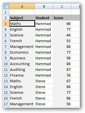
How to Group Rows in Excel Pivot Table (3 Ways) - ExcelDemy Now select any number in the Row Labels of the table. Then right-click and select Group as shown below. Then, enter the Starting ( 60) and Ending ( 100) numbers and the difference ( 10) by which you want to group them. Next, hit OK. Finally, you will see the numbers grouped together as shown in the picture below.👇.

pivot table - Excel PivotTable Remove Column Labels - Super User
How to add column labels in pivot table [SOLVED] Steps:-. Click any date in the Column Lables. Click Pivot table options tab on the Ribbon. In the Options Table, Click Group Field option. Click Months then click Ok. Thats it. check the attached file:-. Attached Files. PIVOT.xlsx (30.3 KB, 6 views) Download.

How to Sort Pivot Table Row Labels, Column Field Labels and Data Values with Excel VBA Macro ...
Excel: How to Sort Pivot Table by Date - Statology Since Excel recognizes the date format, it automatically sorts the pivot table by date from oldest to newest date. However, if we'd like to sort from newest to oldest then we can click on the dropdown arrow next to Row Labels and click Sort Newest to Oldest: The rows in the pivot table will automatically be sorted from newest to oldest:

Quick Pivot Tables in Excel with QuickBooks Data - Export Excel to QuickBooks - Experts in ...
get a row label from pivot table - Microsoft Tech Community Creating PivotTable add data to data model by checking Create PivotTable and after that convert it to cube formulas. Now you may take these formulas and convert it to form you need, for example in H3 it could be =CUBEVALUE( "ThisWorkbookDataModel", CUBEMEMBER("ThisWorkbookDataModel", " [Measures].
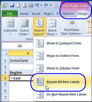
Repeat Pivot Table Labels in Excel 2010 – Excel Pivot Tables
How to Use Label Filters for Text in the Pivot Table? - MS Excel ... When you select the field name, the selected field name will be inserted into the pivot table. Pro Tip. Row Labels are used to apply a filter to rows that have to be shown in the pivot table. By default, it will show you the sum or count values in the pivot table.

How to Do a Pivot Table in Excel
How to reset a custom pivot table row label Now go back to your Pivot and refresh it to find the Problem column and the duplicate column you just made. 5. Enter both fields into the pivot table and you will see the duplicate column has the original values while the Problem column maintains the problem labels. Monday, April 27, 2015 8:39 AM 0 Sign in to vote
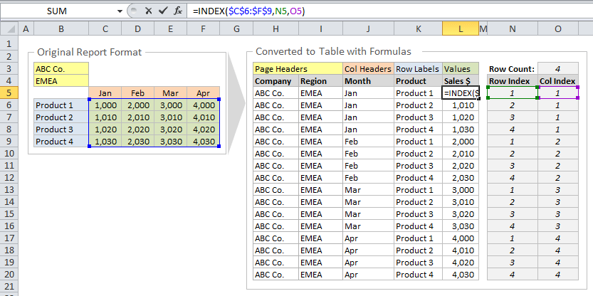
How to Setup Source Data for Pivot Tables - Unpivot in Excel
Excel Pivot Table Filter and Label Formatting - Microsoft Tech Community Excel Pivot Table Filter and Label Formatting Excel 2016 Images of 2 separate workbooks, each with a data table, pivot table and pivot chart, the one on the right created by copy & paste of the one on the left. The one on the right changed: X axis labels on the pivot chart don't have the multi-level option.

ustcer: 23 things you should know about pivot tables
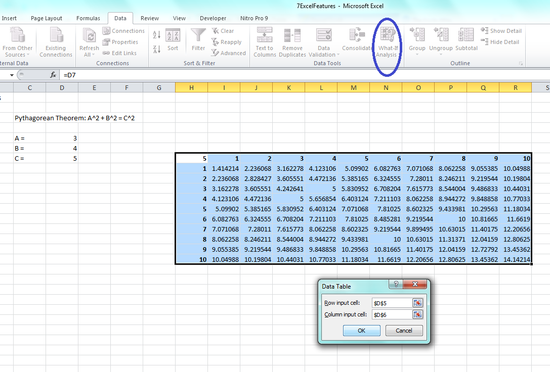
7 Excel Functions and Features to Know

Excel Pivot Table Report - Sort Data in Row & Column Labels & in Values Area, use Custom Lists

Spreadsheet Techie: How to get classic pivot table view in Excel 2010
Post a Comment for "42 excel pivot table labels"